 An
Incomplete Map of the GAN models
An
Incomplete Map of the GAN models
Guo-Jun Qi
Laboratory for MAchine Perception
and LEarning
(MAPLE)
In this short article,
we attempt to plot an incomplete map of the GAN-family models. We focus on the
training criteria of various GAN models, which are not adapted or modified with
any additional features. For this reason, the popular GANs like InfoGAN, conditional GAN and auto-encoder GANs are not
within the scope of our discussion in this article. In particular, we will
review a generalized GAN variant, called GLS-GAN,
which unifies both Wasserstein GAN and
LS-GAN that constitute the second form of regularized GAN models in literature.
Before we move
further, let us take a glance at the map below.
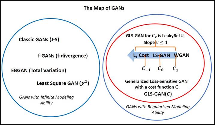
Figure: An incomplete map of GANs.
To plot this map,
we need a criterion to draw the boundary between different GAN models. While
there are many criteria, we classify the GANs into two large classes based on
whether the model has “Regularized versus unregularized
Modeling Ability” [Goodfellow2014].
The unregularized modeling ability (UMA), assumes
that the discriminator of the GAN with UMA can distinguish between real and
fake examples, no matter how these samples are distributed. This is
indeed a non-parametric assumption where the discriminator can be regressed to
any arbitrary form.
In contrast, the
GANs with regularized modeling ability (RMA) resorts to a regularized
model to distinguish between real and fake examples whose distributions satisfy
certain regularity conditions. For example, both LS-GAN [Loss-Sensitive
GAN, Qi2017] and WGAN [Wasserstein GAN, Arjovsky2017] are trained in a space of
Lipschitz continuous functions, which are based on the Lipschitz regularity to
distinguish between real and fake samples [Qi2017].
The significance
of UMA and RMA is they are assumed explicitly or implicitly in theoretical
analysis to prove the consistency conjecture of a proposed GAN model,
which is the density of their generated samples match the density of true
samples.
It has been shown
[Qi2017] that both LS-GAN and WGAN are based on the Lipschitz regularity, an
assumption that the model has regularized modeling ability in contrast to the non-parametric
assumption of unregularized modeling ability
used.
Class 1: Unregularized Modeling Ability (UMA)
The first class of
unregularized
GANs contain the classic GAN [Goodfellow2014], EBGAN [Zhao2016], least-square
GAN [Mao2017] and f-divergence GAN [Nowozin2016].
In [Arjovsky2017],
it has been shown that the classic GAN and EBGAN attempt to minimize J-S
distance and total variation distance between the generative density and the
true data density, while the Least Square GAN is formulated to minimize their
Pearson ![]() divergence and the f-divergence GAN minimizes a
family of f-divergence.
divergence and the f-divergence GAN minimizes a
family of f-divergence.
Table: GANs with UMA and the distance between
distributions they minimize to learn the generator.
|
GANs with UMA |
Distance
between distributions |
|
The classic GAN |
J-S distance |
|
EBGAN |
Total Variation |
|
Least
Square GAN |
|
|
f-GAN |
f-divergence |
Vanishing
Gradient: What is
interesting is these unregularized modeling ability
GANs all suffer from the vanishing gradient problem as discussed in
[Arjovsky2015].
If the manifold of
real data and the manifold of generated data has no or negligible overlap, the
distances they are posed to minimize will become a constant causing vanishing
gradient that cannot update the generator at all. This is a problem that has
been reported in [Goodfellow2013] since the first GAN (J-S) was proposed.
Intractable Sample Complexity: It is particularly worth noting that the unregularized GANs usually require an intractable number of
training samples to reach a satisfactory accuracy in generating samples
indistinguishable from real ones [Arora2017, Qi2017]. In other words, this
implies unregularized GANs could be easily overfit to memorize existing samples rather than generalize
to produce new samples, the most sought property we expect over the GAN
models. This inspires us to pursue
an alternative class of regularized GAN models that are more competent in
generalization.
Open Question: Is this only a coincidence between unregularized GANs and vanishing gradient problem? In
other words, does the unregularity inevitably cause vanishing gradient? Can we find some GANs with UMA but
can avoid the vanishing gradient problem? Probably.
Class 2:
Regularized Modeling Ability (RMA)
On the contrary,
the second class of GANs contain the WGAN and LS-GAN recently developed.
By chance, both models are built based on Lipschitz regularities [Qi2017], and
they do not need unregularzied modeling ability to
prove the consistency conjecture.
Even more, in
[Qi2017], it is shown that both WGAN and LS-GAN belong to a super class of
Generalized LS-GAN (GLS-GAN):
1. WGAN is the GLS-GAN with a cost of ![]() ,
,
2. LS-GAN is the GLS-GAN with a
cost of ![]() .
.
More GLS-GANs can
be found by defining a proper cost function satisfying some conditions
[Qi2017].
An interesting
example is when ![]() , it will define a GLS-GAN with a L1
cost that minimizes the difference between the loss functions of real and
generated samples (up to their margin). This is quite different from the idea
behind both LS-GAN and WGAN, but preliminary results show that it works!
, it will define a GLS-GAN with a L1
cost that minimizes the difference between the loss functions of real and
generated samples (up to their margin). This is quite different from the idea
behind both LS-GAN and WGAN, but preliminary results show that it works!
For details,
please refer to Appendix D of [Qi2017].
Obviously, there
should exist the other GANs with RMA, but not belonging to the GLS-GAN.
More research efforts deserve to discover more GANs with RMA that can properly
regularize the data generation process by introducing priors characterizing the
true data distribution beyond the Lipschitz assumptions. This should be an
interesting direction to expand the territory of the GANs.
Examples of
GLS-GAN (Generalized LS-GAN)
We can adopt a
cost function of Leaky Linear Rectifier ![]() to define the GLS-GAN with a slope
to define the GLS-GAN with a slope ![]() . Then WGAN is GLS-GAN with
. Then WGAN is GLS-GAN with ![]() and LS-GAN is GLS-GAN with
and LS-GAN is GLS-GAN with ![]() .
.
Results on Generalization Performances
To compare the
generalization performance among different GANs, we propose a new metric called
Minimum Reconstruction Error (MRE). The idea is to split dataset into three
parts: training, validation and test.
We use training set to train different GANs, and tune their hyperparameters (including learning rate, when to stop
training iterations) on a validation set.
Then on the test set, for a given sample x, we aim to find an optimal z
that can reconstruct x as much as
possible. That is done by defining ![]()
Clearly, if the
generator G is adequate to produce new samples, it should have a small
reconstruction error on generating unseen examples on a separate test set. Our
experiment results on CIFAR-10 and tiny ImageNet show that regularized models
outperform the unregularized GAN in MRE.
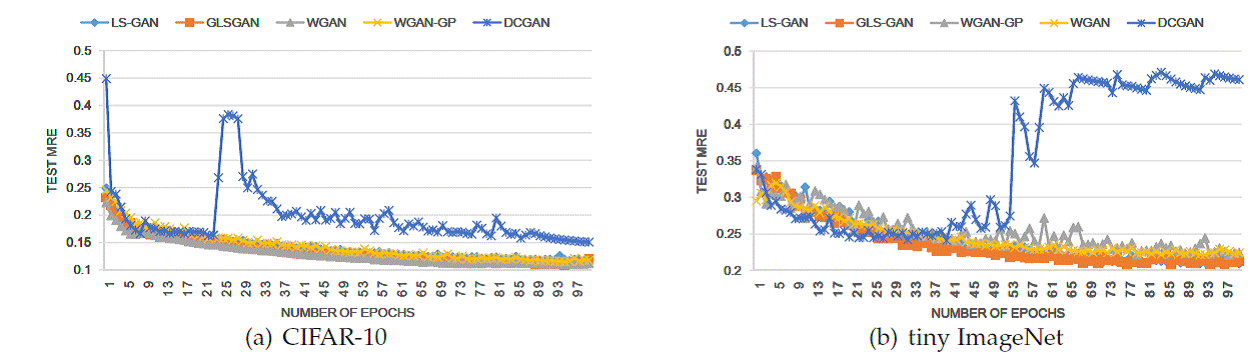
Figure: The change of test
MREs on CIFAR-10 and tiny ImageNet over epochs.
Moreover, as
illustrated below, among regularized GANs, the GLS-GAN has the smallest MRE.
This is not a surprising result, since these regularized GANs, including
LS-GAN, WGAN and WGAN-GP, are only special cases of GLS-GAN. More results can
be found in [Qi2017].
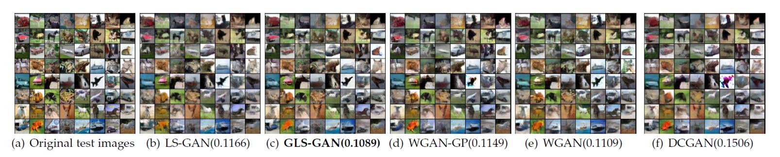
Figure: The images
reconstructed by various GANs on CIFAR-10 with their MREs on the test set in
parentheses.
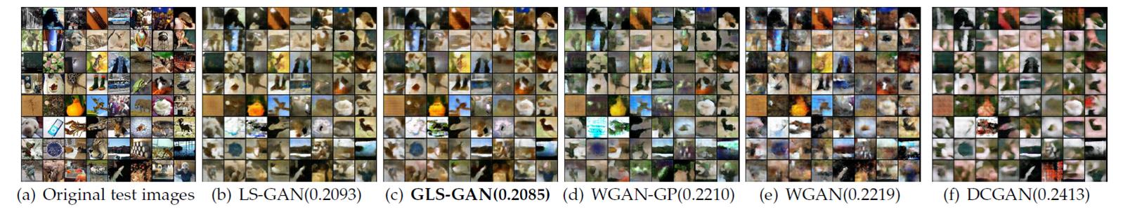
Figure: The images
reconstructed by various GANs on tiny ImageNet with their MREs on the test set
in parentheses.
Source Codes
We have
implemented the GLS-GAN in both pytorch, and tensorflow at our lab github
homepage https://github.com/maple-research-lab
.
Pytorch version: https://github.com/maple-research-lab/glsgan-gp
Tensorflow version: https://github.com/maple-research-lab/lsgan-gp-alt
Original Torch version: https://github.com/maple-research-lab/glsgan
In the GLS-GAN, we
can run both LS-GAN and WGAN as its special cases. More details about GLS-GAN
can be found at [Qi2017].
References
[Qi2017] G.-J. Qi,
Loss-Sensitive Generative Adversarial Networks, preprint, 2017.
[Goodfellow2013]
I. Goodfellow, J. Pouget-Abadie,
M. Mirza, B. Xu, D. Warde-Farley, S. Qzair, A. Courville and Y. Bengio, Generativ Adversarial
Nets, in Advances in Neural Information Processing Systems, 2014, pp.
2672-2680.
[Arjovsky2015] M. Arjovsky and L. Bottou. Towards
Principled Methods for Training Generative Adversarial Networks, 2015.
[Nowozin2016] S. Nowozin, B. Cseke, and R. Tomioka, f-GAN: Training Generative Neural Samplers using Variational Divergence Minimization, 2016.
[Arjovsky2017] M. Arjovsky, S. Chintala, and L. Bottou. Wasserstein GAN, 2017.
[Zhao2016] J.
Zhao, M. Mathieu, and Y. LeCun, Energy-based
Generative Adversarial Network, 2016.
[Mao2017] X. Mao,
Q. Li, H. Xie, R. Y.K. Lau and Z. Wang, Least Squares
Generative Adversarial Networks, 2017.
[Arora2017] S.
Arora, R. Ge, Y. Liang, T. Ma and Y. Zhang, Generalization and Equilibrium in
Generative Adversarial Nets, 2017.
Updated on March 4th 2018
©MAPLE Research